4   Asymptotic hypothesis tests

• 4.1   z-score and t-score
• 4.2   Pearson's chi-squared test
• 4.3   The likelihood ratio test

Asymptotic hypothesis tests address two problems of the exact tests: (i) their numerical complexity and (ii) the difficulty of defining more "extreme" outcomes. Instead of the exact p-value, they use a much simpler equation called a test statistic. This statistic is chosen in such a way that its distribution under the null hypothesis converges to a known limiting distribution for large samples (N → ∞). The limiting distribution can then be used to derive an approximate p-value corresponding to the observed value of the test statistic.⁽¹⁾ Association measures based on asymptotic hypothesis tests often use the test statistic itself as an association score because of its convenience. When converted into a p-value, the score can directly be compared with those of the exact hypothesis tests.

4.1   z-score and t-score

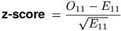
The z-score measure provides a simple solution to problem (i). It is an asymptotic version of the binomial test, based on a normal approximation to the binomial distribution of X₁₁. The test statistic shown below converges to a standard normal distribution for large N and is traditionally called a z-score. It was used by Dennis (1965, 69) to identify "significant word-pair combinations" in a text collection running up to nearly 4 million words.

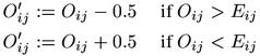
One problem of the z-score measure is its use of the continuous normal distribution to approximate a discrete (binomial) distribution. Yates' continuity correction (Yates, 1934) improves this approximation by adjusting the observed frequencies according to the following rules. Yates' correction can be applied to all cells of the contingency table, although only O₁₁ is relevant for the z-score measure.

When the expected cooccurrence frequency E₁₁ (under H₀) is small, z-score values can become very large, leading to highly inflated scores for low-frequency pair types. The cause of this problem can be traced back to the denominator of the z-score equation, where E₁₁ is the (approximate) variance of X₁₁ under the point null hypothesis of independence. Church et al. (1991) obtain better results from Student's t-test, where this variance is estimated from the sample rather than derived from H₀. In analogy to the z-score, the resulting test statistic is called a t-score.

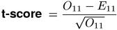
From a theoretical perspective, Student's test is not applicable in this situation. It is designed for a sample of n independent normal variates (from the same distribution). The null hypothesis is a condition on the mean of the normal distribution, while its variance is estimated from the sample. The test statistic of Student's test has a t distribution with n-1 degrees of freedom. There are two ways in which this test can be applied to the comparison of O₁₁ with E₁₁: (a) the "sample" consists of a single item X₁₁ (n=1), which has an approximate normal distribution; or (b) the "sample" consists of N indicator variables, one for each pair token (n=N). In case (a), it is impossible to estimate the variance from a sample of size one. In case (b), the sample variance can be estimated and corresponds to the value used by Church et al. (1991, Sec. 2.2) (O₁₁ is a good approximation of the correct sample variance). However, the individual random variates of this "sample" are indicator variables with only two possible values 0 and 1 (and they are usually highly skewed towards 0). The normal approximation required by the t-test is highly questionable for such binary variables. Following the reasoning of approach (b), the test statistic has a t distribution with N-1 degrees of freedom (Weisstein, 1999, s.v. Student's t-Distribution). Since N is usually large, this distribution is practically identical to the standard normal distribution. The p-values computed in this way are extremely conservative (e.g. compared to Fisher). Surprisingly, the t-score measure performs quite well in collocation extraction tasks (cf. Evert & Krenn, 2001). It may thus be more appropriate to interpret it as a heuristic variant of z-score that avoids the characteristic over-estimation bias of the latter.

Both z-score and t-score are one-sided measures. Large positive values indicate significant evidence for positive association, while large negative values indicate evidence for negative association.

4.2   Pearson's chi-squared test

Other asymptotic hypothesis tests, which are not solely based on O₁₁, also provide a solution to problem (ii) mentioned at the beginning of this section. The p-value corresponding to the observed score g of a test statistic is an approximation to the total probability of all contingency tables that would lead to a score greater than or equal to g. Therefore, the choice of a test statistic defines an explicit ranking of the possible contingency tables. There is no ideal statistic that would follow from a mathematical argument: its definition is a choice that has to be made by the researcher, guided by intuition and common sense.⁽²⁾

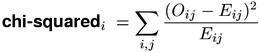
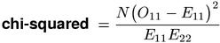
In mathematical statistics, the standard (asymptotic) test for independence in a 2-by-2 contingency table is Pearson's chi-squared test. Its test statistic is based on a comparison of the observed frequencies O_ij with the expected frequencies E_ij under the point null hypothesis of independence, and can be understood as a kind of mean squared error (scaled by the expected variances of the cell frequencies). Edmundson (1965) suggested a "correlation coefficient for events", which is identical to the chi-squared_i formula for the events {U = u} and {V = v} (cf. Section 1). In the same year, Dennis (1965, 69) considers Pearson's test for the extraction of "significant" cooccurrences, but finds the t-score measure more useful.

Pearson's chi-squared test can also be used to compare the success probabilities of two independent binomial distributions, with the null hypothesis of equal success probabilities (sometimes called a 2-by-2 comparative trial). Since the conditional sampling distribution for contingency tables with fixed column (or row) sums is the product of two binomial distributions this version of the chi-squared test can also be applied to the homogeneity of rows (or columns) in a contingency table.

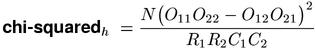
Both versions of Pearson's chi-squared test have been applied to coocurrence data and can be found in the literature (e.g. Manning & Schütze, 1999, Ch. 5). Although it is not at all obvious, the equations given as chi-squared_i (i = independence test) and chi-squared_h (h = homogeneity test) above compute identical association scores. A simpler "normal form" of the test statistic is shown below. It is the recommended standard version of the chi-squared measure.⁽³⁾

For large samples, the test statistic of Pearson's chi-squared test has an asymptotic χ² (chi-squared) distribution with one degree of freedom. The test is two-sided with non-negative association scores. A one-sided test can be obtained by changing the sign of the test statistic when O₁₁ < E₁₁, indicating negative association. The signed square root of the chi-squared measure has an asymptotic standard normal distribution, from which one-sided p-values can be obtained.

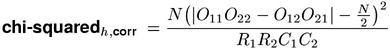
The theoretical background of Pearson's chi-squared test involves a normal approximation to the multinomial sampling distribution. Just as with the z-score measure, Yates' continuity correction should be applied in order to improve the accuracy of the approximation. Note that all four observed frequencies O_ij have to be modified before the statistic is computed. The homogeneity version chi-squared_h has a special form that incorporates Yates' correction (so that the observed frequencies need not be modified). This special form, shown here as the chi-squared_h,corr measure, is often used in applications.

4.3   The likelihood ratio test

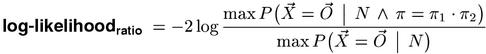
In contrast to Pearson's test with its explicit ranking of contingency tables (based on the "distance" between the tables of observed and expected frequencies), likelihood ratio tests derive their ranking from the sampling distribution: the smaller the probability of a sample outcome under the null hypothesis, the more "surprising" it is and the more evidence against H₀ it provides. When the null hypothesis is not simple, any free parameters are chosen so as to maximise the likelihood of the observed contingency table (the max in the numerator), and the resulting value is scaled by the unconstrained maximum likelihood of the table (the max in the denominator). When the null hypothesis is true, the test statistic shown below (the natural logarithm of the likelihood ratio multiplied by -2) has an asymptotic χ² (chi-squared) distribution, with one degree of freedom in the case of cooccurence data.⁽⁴⁾

The denominator is always maximised by the maximum-likelihood estimates of the probability parameters (because this is the defining criterion of maximum-likelihood estimates). In the case of cooccurrence data, the numerator happens to be maximised by the same estimates for π₁ and π₂ (which is not true in general), and evaluates to the likelihood of the observed contingency table under the point null hypothesis. Inserting explicit expressions for the two maximal probabilities above, we obtain the standard form of the log-likelihood association measure.

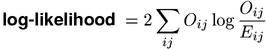
Note that the logarithm is undefined when there are empty cells (with O_ij = 0). For such cells, the entire term evaluates to zero (because 0 * log(0) = 0 by continuous extension) and can simply be omitted from the summation.

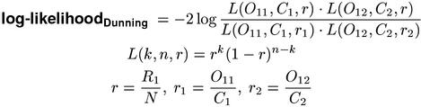
In mathematical statistics, the chi-squared measure is the preferred test for independence in contingency tables because it gives a better approximation to the limiting χ² distribution for small samples (Agresti, 1990, p.49). With the help of numerical simulations, Dunning (1993) showed that the situation is different for the highly skewed tables that are characteristic of cooccurrence data (with O₁₁ small and large sample size N). Here, the accuracy of the log-likelihood measure is much better than that of Pearson's test. Dunning applied the likelihood-ratio test to a contingency table with fixed column sums (i.e. a comparison of two independent binomial distributions, cf. chi-squared_h), leading to the unwieldy an numerically problematic equations shown below (which compute the same association scores as the standard form).

Since the log-likelihood statistic has an asymptotic χ² (chi-squared) distribution, its scores can directly be compared with those of the chi-squared measure. Note that Yates' continuity correction is never applied to likelihood ratio tests. The log-likelihood measure is two-sided and can be converted into a one-sided measure in the same manner as chi-squared above (the signed squared root of the association scores has an asymptotic standard normal distribution under H₀).

Numerical simulation shows that log-likelihood is much more conservative than chi-squared and gives an excellent approximation to the exact p-values of the Fisher measure. Therefore, it has generally been accepted as an accurate and convenient standard measure for the significance of association.